Parameter and configuration Files
When running simulations from yaml and csv files, there are four configuration files that must be used.
The outermost parameter file is the obsparam_*.yaml, which is parsed by
pyuvsim.simsetup.initialize_uvdata_from_params() into a pyuvdata.UVData object,
a beam dictionary, and a pyuvsim.BeamList object.
The antenna layout and telescope config yaml files determine the full properties of the array, including location, beam models, layout, and naming.
The catalog text files give point source lists.
These files contain overall simulation parameters. See Running a simulation for details on how these are passed into a simulation.
filing:
  outdir: '.'   #Output file directory
  outfile_prefix: 'sim' # Prefix for the output file name, separated by underscores
  outfile_suffix: 'results' # Suffix for output file name
  outfile_name: 'sim_results' # Alternatively, give the full name
  output_format: 'uvfits'  # Format for output. Default is 'uvh5', but 'uvfits', measurement sets ('ms'), and 'miriad' are also supported.
  clobber: False        # overwrite existing files. (Default False)
freq:
  Nfreqs: 10    # Number of frequencies
  channel_width: 80000.0    # Frequency channel width
  end_freq: 100800000.0     # Start and end frequencies (Hz)
  start_freq: 100000000.0
  freq_array : [1.0000e+08,   1.0008e+08,   1.0016e+08, 1.0024e+08,
      1.0032e+08,   1.0040e+08,   1.0048e+08, 1.0056e+08,
      1.0064e+08, 1.0072e+08]
  bandwidth: 800000.0
sources:
  catalog: '../pyuvsim/data/gleam_50srcs.vot' # Path to catalog file (txt, vot, skyh5, fhd, etc.) readable with pyradiosky.
  filetype : "gleam" # optionally specify the catalog filetype (skyh5, gleam, vot, text, fhd). If not specified, the code attempt to guess the type.
  spectral_type: flat # If using the GLEAM catalog, specify the spectral type (flat, subband or spectral_index). Defaults to flat.
  table_name: single  # Required for non-GLEAM VO table files
  id_column: name  # Required for non-GLEAM VO table files
  flux_columns: Si  # Required for non-GLEAM VO table files
  ra_column: RAJ2000  # Recommended for non-GLEAM VO table files
  dec_column: DEJ2000  # Recommended for non-GLEAM VO table files
  catalog: 'mock'       # Alternatively, use 'mock' to use a builtin catalog).
  mock_arrangement: 'zenith'    # If using the mock catalog, specify which one. Additional mock keywords are specified here.
  non_nan: 'all'  # Optional, remove source components with NaN Stokes values at all (or any) frequencies
  non_negative: True  # Optional, remove source components with negative Stokes I values
  min_flux: 0.2  # Optional, minimum flux for sourcec components to keep
  max_flux: 1.50  # Optional, maximum flux for sourcec components to keep
telescope:
  array_layout: 'triangle_bl_layout.csv'    # Antenna layout csv file
  telescope_config_name: '28m_triangle_10time_10chan.yaml'  # Telescope metadata file.
time:
  Ntimes: 10        # Number of times.
  integration_time: 11.0  # Time step size  (seconds)
  start_time: 2457458.1738949567    # Start and end times (Julian date)
  end_time: 2457458.175168105
  duration_hours: 0.0276
select: # limit which baselines are simulated. Use any UVData.select keywords (except polarizations) and/or redundant_threshold
  bls: '[(1, 2), (3, 4), (5, 6)]'
  ant_str: 'cross'
  antenna_nums: [1, 7, 9, 15]
  redundant_threshold: 0.1 # redundancy threshold in meters. Only simulate one baseline per redundant group
ordering: # specify the baseline-time order and baseling conjugation convention
  conjugation_convention: ant1<ant2
  blt_order: [time, baseline]
Note The example above is shown with all allowed keywords, but many of these are redundant. This will be further explained below. Only one source catalog will be used at a time.
Filing
Specifies where the results file will be output, what name the file should have, and whether or not to overwrite existing files. None of these parameters are required.
Frequency
As is the standard with
pyuvdata, the frequencies refer to the frequency at the channel center. Thebandwidthrefers to the total band covered by all channels, and the channel width is the separation between channel centers. Therefore, the following relations hold:bandwidth = Nfreqs * channel_width bandwidth = (end_freq + channel_width/2.) - (start_freq - channel_width/2.) = ( end_freq - start_freq) + channel_width start_freq = end_freq - bandwidth + channel_width end_freq = start_freq + bandwidth - channel_widthTime and frequency structure may be defined with different combinations of keywords to suit the user’s purposes. The user must specify sufficient information for the frequency array to be defined.
Minimum frequency requirements:
Specify bandwidth via one of the following combinations:
(
start_freq,end_freq)(
channel_width,Nfreqs)(
bandwidth)Specify channel width via:
(
Nfreqs)(
channel width)Specify a reference frequency via:
(
start_freq)(
end_freq)As long as one of the sets from each category above is met by the supplied keywords, the frequency array will be successfully built. You can also just give an explicit
freq_array.The
channel_widthshould be specified as a scalar unlessfreq_arrayis specified, in which casechannel_widthcan either be a scalar or an array of the same length asfreq_array.If you specify an explicit
freq_arraythat is not evenly spaced or is only length one, you must specify thechannel_width, either as a single value (in Hz) or as an array of the same length asfreq_array.
Time
The time array is specified similarly. The entries in the
time_arrayindicate the center of each time step in Julian date. Theintegration_timeis the time step size in seconds. The user may also specifyduration_hoursorduration_daysto specify the total time covered by all time steps. The following relations among parameters hold:duration_hours = Ntimes * integration_time / (3600.) duration_days = duration_hours / 24. duration_days = (end_time - start_time) + integration_time / 86400 start_time = end_time - duration_days + integration_time / 86400 end_time = start_time + duration_days - integration_time / 86400The numerical factors are to convert among seconds, days, and hours. The user must specify sufficient information for the time array to be defined:
Minimum time requirements:
Total time:
(
start_time,end_time)(
integration_time,Ntimes)(
duration_hours) or (duration_days)Time step:
(
Ntimes)(
integration_time)Reference time:
(
start_time)(
end_time)As long as one of the sets from each category above is met by the supplied keywords, the time array will be successfully built. You can also just give an explicit
time_array.The
integration_timeshould be specified as a scalar unlesstime_arrayis specified, in which caseintegration_timecan either be a scalar or an array of the same length astime_array.If you specify an explicit
time_arraythat is not evenly spaced or is only length one, you must specify theintegration_time, either as a single value (in s) or as an array of the same length astime_array.Note that to get sufficient precision, the parameters that contain absolute times (
start_time,end_time,time_array) must be 64bit floats. As a convenience, atime_offsetparameter can be supplied which will be added to the the parameters that contain absolute times so that those parameters can be written as lower precision numbers. This is needed to support automated generation of parameter yamls as the standard yaml dumpers do not write the full precision of 64bit values.
Telescope Configuration
Under the telescope section, the keywords
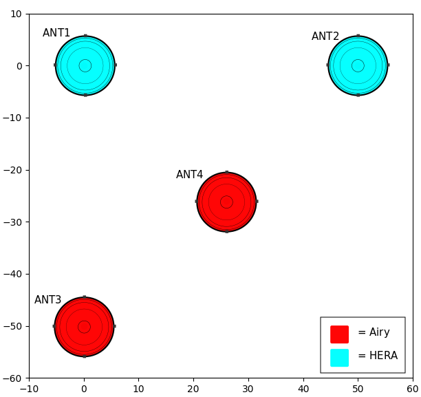
array_layoutandtelescope_config_namegive paths to, respectively, the array layout text file and the telescope metadata configuration yaml file. These path may either be absolute or specified relative to the location of the obsparam yaml file.Example array layout with four antennas:
Name Number   BeamID   E          N          U

ANT1        0        0     0.0000   0.0000  0.0000
ANT2        1        0     50.000   0.0000  0.0000
ANT3        2        2     0.0000   -50.00  0.0000
ANT4        3        2     26.000   -26.00  0.0000
Columns here provide, in order from left to right, the antenna name, antenna number, a beam ID number, and the antenna positions relative to the array center in east, north, up (ENU) in meters. The layout file has a corresponding telescope metadata file, shown below:
beam_paths:
  0:
    filename: hera.beamfits
  1: !UVBeam
    filename: mwa_full_EE_test.h5
    pixels_per_deg: 1
    freq_range: [100.e+6, 200.e+6]
  2: !AnalyticBeam
    class: AiryBeam
    diameter: 16
  3: !AnalyticBeam
    class: GaussianBeam
    sigma: 0.03
  4: !AnalyticBeam
    class: pyuvdata.GaussianBeam
    diameter: 14
spline_interp_opts:
        kx: 4
        ky: 4
freq_interp_kind: 'cubic'
telescope_location: (-30.72152777777791, 21.428305555555557, 1073.0000000093132)
telescope_name: BLLITE
select:
  freq_buffer: 1000000  # 1 MHz either side of simulated frequencies
This yaml file provides the telescope name, location in latitude/longitude/altitude in degrees/degrees/meters (respectively), and the beam dictionary (the
beam_pathssection). In this case we have 5 different types of beams with beam IDs running from 0 to 4:
0: a UVBeam from the file
hera.beamfits1: a UVBeam (for the MWA) with some keywords specified to pass to
UVBeam.read2: an analytic Airy disk with diameter 16 m
3: an analytic Gaussian beam with sigma 0.03 radians (for the E-Field beam)
4: an analytic Gaussian with diameter 14 m
The parameters for each beam depends on whether it is a UVBeam or an analytic beam.
UVBeams can be specified with our without
!UVBeamtag, must have afilenameparameter and can optionally have any other parameter that can be passed to theUVBeam.readmethod. We encourage using the!UVBeamtag unless a globalselectsection is specified (see below).Analytic Beams should use the
!AnalyticBeamtag, must specify theclassparameter and can have parameters specifying shapes as appropriate for their type. Theclassparameter can optionally contain a module name, which allows any properly defined importable analytic beam to be specified. See the pyuvdata documentation on analytic beams to learn how to create new analytic beams.The dictionary only needs to be as long as the number of unique beams used in the array, while the layout file specifies which antennas will use which beam type. This allows for a mixture of beams to be used, as in this example. Unassigned beams will be ignored (the given layout file only uses beamIDs 0 and 2).
Analytic beams may require shape parameters depending on their type. The following types are defined in pyuvdata and are always available:
AiryBeam: Airy disk (ie, diffraction pattern of a circular aperture). Requires an antenna diameter and is inherently chromatic and unpolarized.
GaussianBeam: Gaussian function shaped beam, inherently unpolarized. Requires either an antenna
diameter(in meters) or a standard deviationsigma(in radians). Gaussian beams specified by a diameter will have their width matched to an Airy beam at each simulated frequency, so are inherently chromatic. For Gaussian beams specified withsigma, thesigma_typedefines whether the width specified bysigmaspecifies the width of the E-Field beam (default) or power beam in zenith angle. If onlysigmais specified, the beam is achromatic, optionally both thespectral_indexandreference_frequencyparameters can be set to generate a chromatic beam with standard deviation defined by a power law:stddev(f) = sigma * (f/ref_freq)**(spectral_index)UniformBeam: The same response in all directions, inherently achromatic and unpolarized. No additional parameters.
ShortDipoleBeam: A classical short dipole beam, this is an intrinsically polarized but achromatic analytic beam. No additional parameters.
There are also some global parameters that apply to all the UVBeams:
freq_interp_kindsets the type of frequency interpolation for all UVBeam objects defined in the beam list (see documentation on UVBeam for options).The
spline_interp_optskeyword lets the user set the order on the angular interpolating polynomial spline function. By default, it is cubic.The
selectsection allows for doing partial reading UVBeam files. This can include any selection parameter accepted by UVBeam.read. It can also take afreq_bufferparameter which is used to set thefreq_rangeon read so that only frequencies withinfreq_bufferof the min and max of the simulated frequencies will be read during setup. Using select parameters here or in the individual UVBeam specification above can help reduce peak memory usage. Note that if any of the sameselectparameters are passed for a specific UVBeam and to theselectsection, the values passed for the specific UVBeam will supercede the values in theselectsection, unless the beams are specified using the!UVBeamyaml tag. Note: this global select should not be used if!UVBeamyaml tags are used (as shown in beam 0 in the example yaml). This is because using the!UVBeamyaml tag results in a UVBeam being constructed before the rest of the yaml is read, so any globally specified selects will be done after the read rather than during the read and will be applied in addition to any selects done during the read.The figure below shows the array created by these configurations, with beam type indicated by color.
Telescopes on the Moon
If the
lunarskymodule is installed, thetelescope_locationcan be interpreted as the lon/lat/alt of an observatory on the Moon, defined in the “Mean Earth/ Mean Rotation” frame (see documentation onlunarsky). Setting the keywordworld: moonin the telescope_config file enables this. Optionally set thelunar_ellipsoidkeyword to specify which reference ellipsoid to use (it defaults to “SPHERE”). Must be one of “SPHERE”, “GSFC”, “GRAIL23”, “CE-1-LAM-GEO” (seelunarskypackage for details).beam_paths: 0: !AnalyticBeam class: 'uniform' telescope_location: (0.6875, 24.433, 0) world: 'moon' telescope_name: apollo11
Sources
Specify the path to a catalog file via
catalog. The path can be given as an absolute path or relative to the location of the obsparam. This catalog can be any file type that is readable withpyradiosky. pyradiosky’s SkyModel (SkyModel) supports a wide range of catalogs, including point sources and diffuse maps and multiple spectral models.An example text catalog file:
The columns are:
source_id: Identifier for the source
ra_icrs: Right ascension of source in decimal degrees in the ICRS frame. Other frames are supported, e.g.ra_J2000would yield an FK5 frame at the J2000 epoch. Seepyradioskydocs for more details on frame specification.
dec_icrs: Declination of source in decimal degrees in the ICRS frame. Other frames are supported, e.g.dec_J2000would yield an FK5 frame at the J2000 epoch. Seepyradioskydocs for more details on frame specification.
Flux: Source stokes I brightness in Janskies. (Currently only point sources are supported).
Frequency: A reference frequency for the given flux. This will be used for spectral modeling.If the catalog is a GLEAM VO table file, optionally specify the
spectral_typeas one of:flat,subbandorspectral_index. If not specified it defaults toflat.If the catalog is a different VO table file, several other keywords are required or recommended:
table_name: The name of the table to use from the file (required).
id_column: The name of the column to use for the source IDs (required).
flux_columns: One or a list of columns to use for the source fluxes (a list for fluxes at multiple frequencies) (required).
lon_column: The name of the column to use for the source longitudes (required,ra_columnis a deprecated synonym)
lat_column: The name of the column to use for the source latitudes (required,ra_columnis a deprecated synonym).
frame: The name of theastropyframe to use.Optionally specify the
filetypeas one of [‘skyh5’, ‘gleam’, ‘vot’, ‘text’, ‘fhd’]. If this is not specified, the code attempts to guess what file type it is.Alternatively, you can specify a
mockand provide themock_arrangementkeyword to specify which mock catalog to generate. Available options are shown in thepyuvsim.simsetup.create_mock_catalog()docstring.Flux limits can be made by providing the keywords
min_fluxandmax_flux. These specify the min/max stokes I flux to choose from the catalog.Note that when using the GLEAM catalog, depending on the spectral type you use there can be sources that have Stokes values that are NaNs and Stokes I values that are negative. You can remove sources that have NaN Stokes values at either any or all frequencies using the
non_nankeyword (can be set to “any” or “all”, note that for subband spectral types the default flux interpolation will not result in NaNs as long as not all the Stokes values are NaN). You can remove sources with negative Stokes I values using thenon_negativekeyword (set to True). See pyradiosky documentation for more details.The option
horizon_buffercan be set (in radians) to adjust the tolerance on the coarse horizon cut. After reading in the catalog,pyuvsimroughly calculates the rise and set times (in local sidereal time, in radians) for each source. If the source never rises, it is excluded from the simulation, and if the source never sets its rise/set times are set to None. This calculation is less accurate than the astropy alt/az calculation used in the main task loop, so a “buffer” angle is added to the set lst (and subtracted from the rise lst) to ensure sources aren’t accidentally excluded. Tests indicate that a 10 minute buffer is sufficient. Pyuvsim also excludes sources below the horizon after calculating their AltAz coordinates, which is more accurate. The coarse cut is only to reduce computational load.
Select
Specify keywords to select which baselines to simulate. The selection is done by UVData.select, so it can accept any keyword that function accepts, except ones that affect polarization because pyuvsim computes all polarizations.
Note that if using the
blsparameter for selecting, which specifies a list of baseline tuples, the list needs to be wrapped in a string in the obsparam yaml file.In addition to the UVData.select keywords, a
redundant_thresholdparameter can be specified. If it is present, only one baseline from each set of redundant baselines is simulated. Theredundant_thresholdspecifies how different two baseline vectors can be to still be called redundant – the magnitude of the vector differences must be less than or equal to the threshold. The vector differences are calculated for a phase center of zenith (i.e. in drift mode).
Ordering
Specify how data on the UVData object is ordered.
The baseline conjugation convention (specified as
conjugation_convention) defaults to"ant1<ant2"(which is a change in versions 1.3.1, in earlier versions it defaulted to"ant2<ant1"). If it is set to something other than"ant1<ant2", it is passed to thepyuvdata.UVData.conjugate_bls()method, see those docs for more information.The ordering along the baseline-time axis (specified as
blt_order) defaults to["time", "baseline"](meaning it is ordered first by time and then by baseline number). If it is set to anything else, it is passed to thepyuvdata.UVData.reorder_blts()method, see those docs for more information. Note that the object is required to be in the["time", "baseline"]order for running simulations with the pyuvsim simulator, so if it is set to anything else, the uvdata object will be reordered before the simulation and then ordered back as specified after the simulation is complete.